Fit a Sparse Tensor Decomposition Model

This notebook demonstrates how to fit a sparse tensor decomposition model to data, using the SparseCP class of the Barnacle library. First we’ll generate a simulated data tensor with added noise, then fit a sparse tensor decomposition model to this simulation. We’ll evaluate the result using tools from Barnacle and the tlviz library to compare factor matrices between the model and the simulation ground truth. Finally we’ll explore how multiple random initializations is good practice when fitting CP tensor decomposition models, and can result in improved model solutions.

# imports

import numpy as np
import scipy
import tensorly as tl
import tlviz
from barnacle import (
    SparseCP,
    visualize_3d_tensor,
    simulated_sparse_tensor,
    plot_factors_heatmap
)

# generate simulated data tensor

true_rank = 5
true_shape = [20, 15, 10]
true_densities = [.2, .4, .6]

# re-seed simulated data until all factor matrices are full rank
full_rank = False
while not full_rank:
    # generate simulated tensor
    sim_tensor = simulated_sparse_tensor(
        shape=true_shape,
        rank=true_rank,
        densities=true_densities,
        factor_dist_list=[
            scipy.stats.uniform(loc=-1, scale=2),
            scipy.stats.uniform(),
            scipy.stats.uniform()
        ],
        random_state=9481
    )
    # check that all factors are full rank
    full_rank = np.all([np.linalg.matrix_rank(factor) == true_rank for factor in sim_tensor.factors])

# add 20% noise to simulated dataset
noisy_sim_tensor = sim_tensor.to_tensor(noise_level=0.2, sparse_noise=True, random_state=4791)

# visualize noisy simulated tensor data
fig = visualize_3d_tensor(
    noisy_sim_tensor,
    shell=False,
    midpoint=0,
    show_colorbar=True,
    label_axes=True,
    range_color=[-1, 1],
    opacity=1,
)
fig.show()

# fit sparse tensor decomposition model to simulated data

# instantiate sparse cp model
model = SparseCP(
    rank=5,
    lambdas=[0.4, 0, 0],
    nonneg_modes=[1, 2],
    random_state=72258
)

# fit model to data
cp = model.fit_transform(noisy_sim_tensor, verbose=3)

Beginning initialization 1 of 1
loss: 18.26476536487174
loss: 7.390206063801999
loss: 7.023123827077382
loss: 7.011798742456526
loss: 7.011523418863808
loss: 7.011422224375263
loss: 7.011348799819072
loss: 7.011275583735396
loss: 7.0111964079706794
loss: 7.011110165842045
loss: 7.011016398799992
loss: 7.010914197193543
loss: 7.010803097188486
loss: 7.010682594299325
loss: 7.010552363496999
loss: 7.01041193663957
loss: 7.010260864275709
loss: 7.010098858630826
loss: 7.009925489797718
loss: 7.009741483281008
loss: 7.009547323999183
loss: 7.009343444840475
loss: 7.009130401361401
loss: 7.008909225955648
loss: 7.008666501146237
loss: 7.008391447615166
loss: 7.008081409998965
loss: 7.007735817511848
loss: 7.007354122148607
loss: 7.00693784146193
loss: 7.006490258340945
loss: 7.006015720793433
loss: 7.005518412423505
loss: 7.005004394257134
loss: 7.004483809984444
loss: 7.0039648940689725
loss: 7.003452579179688
loss: 7.002967257596921
loss: 7.00255241799881
loss: 7.002300180799768
loss: 7.002096457474012
loss: 7.001936496562364
loss: 7.0017964377290465
loss: 7.001662987886994
loss: 7.001539333625742
loss: 7.001426988364198
loss: 7.001325628882855
loss: 7.001233712868817
loss: 7.001185273216217
loss: 7.00118397780891
Algorithm converged after 50 iterations

Great, the algorithm converged and we have a fit model!

Now we can compare how well the factor matrices of our fit model match the ground truth factor matrices used to generate the simulated data. We’ll do this in two ways:

1. We’ll calculate a factor match score that quantifies the similarity of the two sets of factors. This is accomplished using the factor_match_score function from the tlviz Python library (part of the Tensorly ecosystem). A score of 1 indicates identical factor matrices, whereas a score of 0 indicates complete dissimilarity.

2. We’ll visually compare the two sets of factor matrices using the plot_factors_heatmap function of the Barnacle library.

Note that in CP tensor decompositions, the order of factors is arbitrary. So for both comparisons, we first have to permute the components (factor matrix columns) so that we are comparing the most similar components between models.

# compare factor matrices of the model to those used to generate the simulation

# calculate factor match score (FMS) between two sets of factor matrices
fms, permutation = tlviz.factor_tools.factor_match_score(
    sim_tensor,
    cp,
    return_permutation=True
)
print(f'The FMS between model and simulation factor matrices is: {fms:.2f}')

# permute model components to align with simulation components
permuted_cp = tlviz.factor_tools.permute_cp_tensor(cp, permutation)

# plot factor heatmaps
heatmap_params = {'vmin':-1, 'vmax':1, 'cmap':'seismic', 'center':0}
fig, ax = plot_factors_heatmap(
    tl.cp_normalize(permuted_cp).factors,
    reference_factors=tl.cp_normalize(sim_tensor).factors,
    mask_thold=[0, 0],
    ratios=True,
    heatmap_kwargs=heatmap_params
)
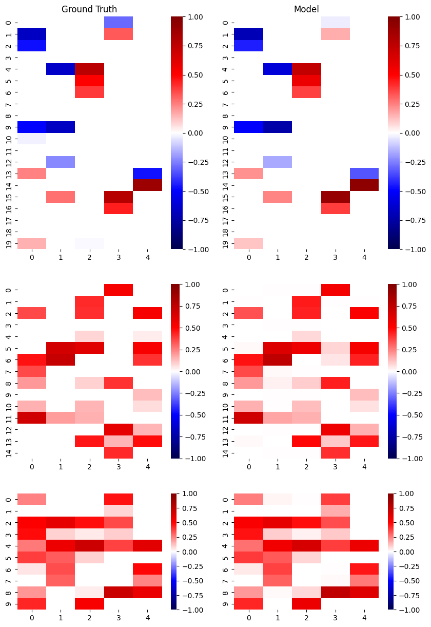
ax[0][0].set_title('Ground Truth');
ax[0][1].set_title('Model');

The FMS between model and simulation factor matrices is: 0.57

Ok so the FMS between the model and simulation is 0.57 – not terrible, but not great. And visually comparing the two sets of factor matrices we can see some similarities, but also some places where the model weights diverge significantly from the simulation ground truth. To improve the model, some more information about CP models could be helpful.

CP models are fit by solving a non-convex optimization problem. This means that even if the algorithm converges, it is possible it converged on a local minimum that doesn’t represent the overall best solution to the problem. Therefore in practice, it is common to fit several models with different random initializations, and select the solution that results in the lowest error as the overall best fit model. We can also compare the solutions between initializations to increase confidence in the selected solution.

# fit sparse tensor decomposition model to simulated data, with 10 random initializations

# instantiate sparse cp model
model2 = SparseCP(
    rank=5,
    lambdas=[0.4, 0, 0],
    nonneg_modes=[1, 2],
    random_state=72258,
    n_initializations=10
)

# fit model to data
cp2 = model2.fit_transform(noisy_sim_tensor, verbose=2)

Beginning initialization 1 of 10
Algorithm converged after 50 iterations

Beginning initialization 2 of 10
Algorithm converged after 19 iterations

Beginning initialization 3 of 10
Algorithm converged after 75 iterations

Beginning initialization 4 of 10
Algorithm converged after 31 iterations

Beginning initialization 5 of 10
Algorithm converged after 11 iterations

Beginning initialization 6 of 10
Algorithm converged after 10 iterations

Beginning initialization 7 of 10
Algorithm converged after 33 iterations

Beginning initialization 8 of 10
Algorithm converged after 7 iterations

Beginning initialization 9 of 10
Algorithm converged after 43 iterations

Beginning initialization 10 of 10
Algorithm converged after 31 iterations

# compare solutions between initializations

fig, ax = tlviz.visualisation.optimisation_diagnostic_plots(
    model2.candidate_losses_,
    n_iter_max=100
)
ax[0].set_ylabel('Loss');
ax[1].set_ylabel('Loss (Log scale)');

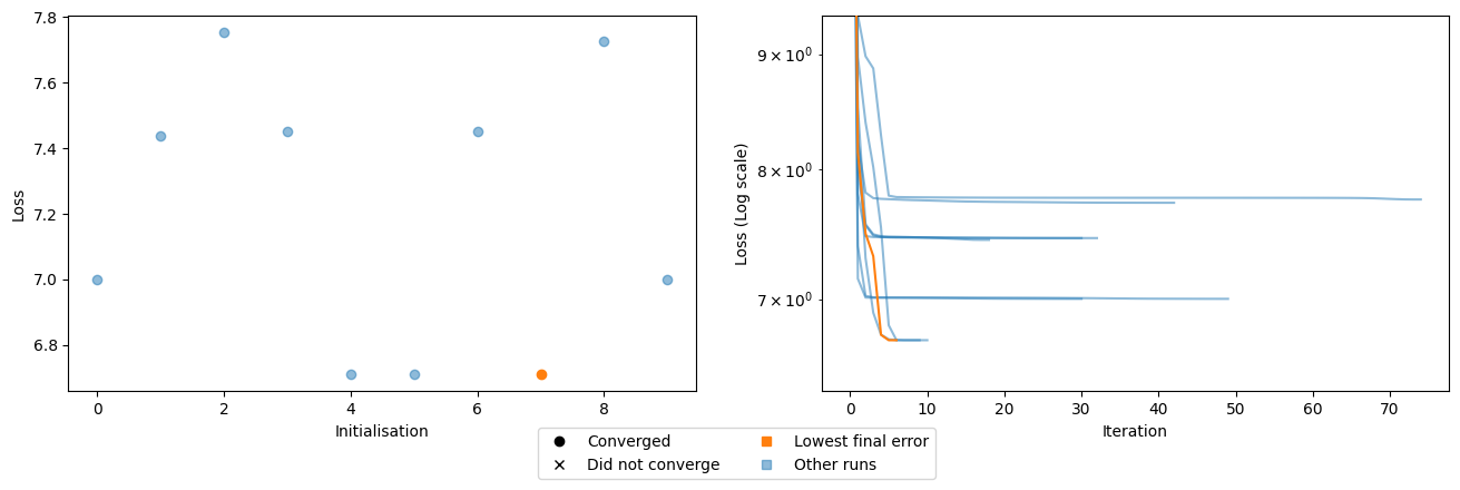
It looks like all 10 initializations converged, and there were a range of different solutions. Two independent random initializations both converged with a losses around 7.75, suggesting this may represent a local minimum. We see other potential minima where multiple initializations all converged around a similar loss value, such as ~7.45 (three initializations), and ~7.0 (two initializations). The best model is one of three that settled around a loss of 6.7, with the lowest loss solution converging in just 7 iterations.

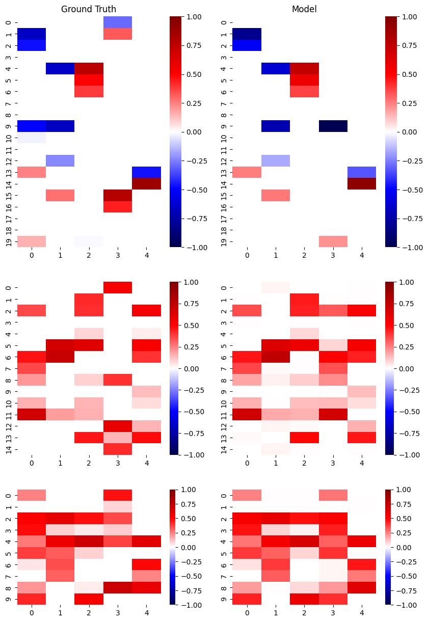
Next we’ll again compare the factor matrices from this lowest loss model to the ground truth simulation. We’ll see that multiple initializations resulted in a model that more closely matches ground truth, both in terms of FMS score and visual comparison of the factor matrices.

# compare factor matrices of the model to those used to generate the simulation

# calculate factor match score (FMS) between two sets of factor matrices
fms2, permutation2 = tlviz.factor_tools.factor_match_score(
    sim_tensor,
    cp2,
    return_permutation=True
)
print(f'The FMS between model and simulation factor matrices is: {fms2:.2f}')

# permute model components to align with simulation components
permuted_cp2 = tlviz.factor_tools.permute_cp_tensor(cp2, permutation2)

# plot factor heatmaps
heatmap_params = {'vmin':-1, 'vmax':1, 'cmap':'seismic', 'center':0}
fig, ax = plot_factors_heatmap(
    tl.cp_normalize(permuted_cp2).factors,
    reference_factors=tl.cp_normalize(sim_tensor).factors,
    mask_thold=[0, 0],
    ratios=True,
    heatmap_kwargs=heatmap_params
)
ax[0][0].set_title('Ground Truth');
ax[0][1].set_title('Model');

The FMS between model and simulation factor matrices is: 0.74